Simple discrete fourier transformation in Swift

Fourier transformation is a mathematical operation that can be used to decompose a signal into its frequency components. It is used in many fields, for example in signal processing, image processing, and in physics. It is also used in cryptography, for example in the RSA algorithm.

Discrete Fourier transformation (DFT) is a special case of the Fourier transformation. It is used to decompose a signal that is sampled at discrete points in time. When using digital singnals on computers, this is always the case.

The theory behind fourier transfomation is that any signal can be expressed as a (potentially infinite) sum of sin and cos functions. For each of the frequency components, we want to fond the amplitude and the phase.

In this post, I will explain step by step how I implemented

To get started, I created a data structure to represent the different signal parts consisting of frequency, amplitude, and phase:

struct SignalPart {
    let frequency: Double
    let amplitude: Double
    let phase: Double
}

Generating a signal

The next step is to create a function to generate the signal. Becuase all of this only works for discrete signals, we need to sample the signal at discrete points in time. The sampling rate is the number of samples per second. As we want to use the signal for testing, we need to be able to generate a signal with a known frequency. The function generateDiscreteSignal takes the sampling rate, the duration, and the signal parts as parameters. It returns an array of samples.

func generateDiscreteSignal(numberOfSamplesPerSecond: Int, seconds: Double, signalParts: [SignalPart]) -> [Double] {
    let numberOfSamples = Int(Double(numberOfSamplesPerSecond) * seconds)
    return (0..<numberOfSamples)
        // Calculate the timestamp for each sample
        .map { Double($0) / Double(numberOfSamples - 1) * Double(seconds) }
        // Calculate the signals value fot each timestamp
        .map { (time: Double) -> Double in
            // To calculate the signal value, sum up the values of the different signal parts
            signalParts
                .map { (signalPart: SignalPart) -> Double in
                    sin((signalPart.frequency * time + signalPart.phase) * 2 * Double.pi) * signalPart.amplitude
                }
                .reduce(0, +)
        }
}

Now, we can generate a signal with a known frequency. For example, we can generate a signal with a frequency of 1 Hz and an amplitude of 1 combined with a signal with a frequency of 5 Hz and an amplitude of 0.1 and a phase of 0.25 (shifted by \(0.25 \cdot 2 \pi = 90^{\circ}\)):

let signal = generateDiscreteSignal(numberOfSamplesPerSecond: 50, seconds: 1, signalParts: [
    SignalPart(frequency: 1, amplitude: 1, phase: 0),
    SignalPart(frequency: 5, amplitude: 0.1, phase: 0.25)
])

To check if this is working, we can use Swift Playgrounds build in function to plot signals. To make Swift Playgrounds numbers as a graph, the code must itterate over the values which can easily be accomplished using a simple map: signal.map() { $0 }. The result is the following graph:

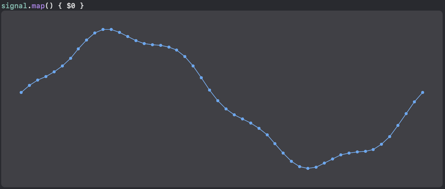
As you can see, the signal consists of two parts with different frequencies. The first part has a frequency of 1 Hz and the second part has a frequency of 5 Hz. The second part is shifted by 90 degrees.

Discrete Fourier transformation

Now that we have a signal, we can use the discrete fourier transformation to decompose it into its frequency components. I don’t want to go into the details of the fourier transformation here, as there are already very good explanations on the internet. For example, the video The Algorithm That Transformed The World from Veritasium is a very good visual explenation and was the inspiration for this post.

The base idea of the algorithm is to multiply the signal with many pure sine and cosine functions with only one frequency. If the signal contains a component of that frequency, the result is non-zero. If the signal does not contain the frequency, the result is zero. Using that knowledge, we can implement the algorithm. The issue with this algorithm is that it is very inefficient. It has a time complexity of O(n^2). This means that it takes n^2 time to calculate the transformation for a signal with n samples. If we already know that we only want to have a look at the first k frequency components, we can limit this in the algorithm to only calculate the first k frequency components. This will reduce the time complexity to O(kn). In the follwing example, I set k to 15.

func discreteFourierTransform(signal: [Double], durationInSeconds: Int) -> [SignalPart] {
    let baseFrequency = 1 / Double(durationInSeconds)
    // To calculate all possible frequencies, use the following
    // let frequencies = (0..<signal.count)
    let frequencies = (0..<15)
        .map { Double($0) * baseFrequency }

    let signalParts = frequencies.map { frequency in

        let sinPart = signal.enumerated().map { index, value -> Double in
            let time = Double(index) / Double(signal.count - 1) * Double(durationInSeconds)

            return value * sin(frequency * time * 2 * Double.pi)
        }
            .reduce(0, +)

        let cosPart = signal.enumerated().map { index, value -> Double in
            let time = Double(index) / Double(signal.count - 1) * Double(durationInSeconds)

            return value * cos(frequency * time * 2 * Double.pi)
        }
            .reduce(0, +)

        // Calculate combined sine wave
        let amplitude = sqrt(cosPart*cosPart+sinPart*sinPart)
        let phase = atan2(cosPart, sinPart) / (2 * Double.pi)

        return SignalPart(frequency: frequency, amplitude: amplitude, phase: phase)
    }

    // Normalize amplitude
    return signalParts.map {
        SignalPart(frequency: $0.frequency, amplitude: $0.amplitude / Double(signal.count - 1) * 2, phase: $0.phase)
    }
}

Now, we can use the function to calculate the frequency components of the signal we generated before:

let detectedFrequncies = discreteFourierTransform(signal: signal, durationInSeconds: 1)

Using the same method as above, we can plot the amlitude of the frequency components:

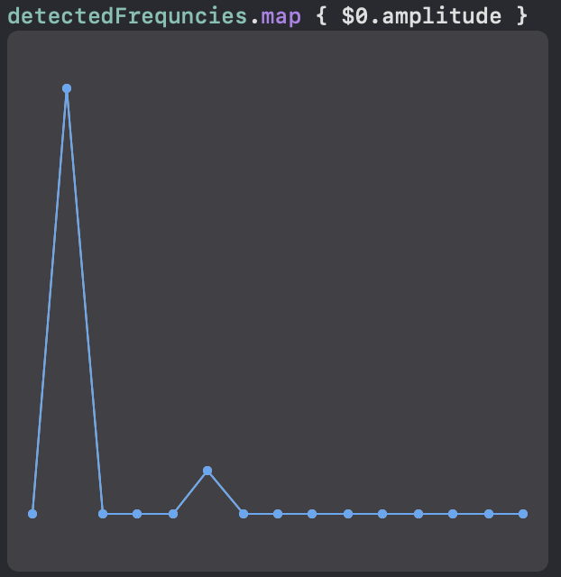
As you can see, the algorithm detected the two frequencies we used to generate the signal with their respective amplitudes.